A Background and Basic Concepts

This Appendix describes:

The overall structure of our Docker-based PostgreSQL sandbox

Basic concepts around each of the elements that make up our sandbox: tidy data, pipes, Docker, PostgreSQL, data representation, and our petsqlr package.

A.1 The big picture: R and the Docker / PostgreSQL playground on your machine

Here is an overview of how R and Docker fit on your operating system in this book’s sandbox:

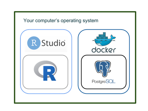
R and Docker

You run R from RStudio to set up Docker, launch PostgreSQL inside it and then send queries directly to PostgreSQL from R. (We provide more details about our sandbox environment in the chapter on mapping your environment.

A.2 Your computer and its operating system

The playground that we construct in this book is designed so that some of the mysteries of accessing a corporate database are more visible – it’s all happening on your computer. The challenge, however, is that we know very little about your computer and its operating system. In the workshops we’ve given about this book, the details of individual computers have turned out to be diverse and difficult to pin down in advance. So there can be many issues, but not many basic concepts that we can highlight in advance.

A.3 R

We assume a general familiarity with R and RStudio. RStudio’s Big Data workshop at the 2019 RStudio has an abundance of introductory material (Ruiz 2019).

This book is Tidyverse-oriented, so we assume familiarity with the pipe operator, tidy data (Wickham 2014), dplyr, and techniques for tidying data (Wickham 2018).

R connects to a database by means of a series of packages that work together. The following diagram from a big data workshop at the 2019 RStudio conference shows the big picture. The biggest difference in terms of retrieval strategies is between writing dplyr and native SQL code. Dplyr generates SQL-92 standard code; whereas you can write SQL code that leverages the specific language features of your DBMS when you write SQL code yourself.

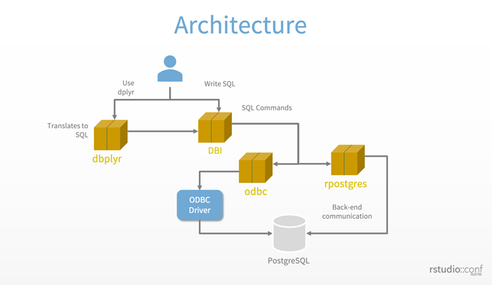
Rstudio’s DBMS architecture - slide # 33

A.4 Our `sqlpetr` package

The sqlpetr package is the companion R package for this database tutorial. It has two classes of functions:

Functions to install the dependencies needed to build the book and perform the operations covered in the tutorial, and
Utilities for dealing with Docker and the PostgreSQL Docker image we use. sqlpetr has a pkgdown site at https://smithjd.github.io/sqlpetr/.

A.5 Docker

Docker and the DevOps tools surrounding it have fostered a revolution in the way services are delivered over the internet. In this book, we’re piggybacking on a small piece of that revolution, Docker on the desktop.

A.5.1 Virtual machines and hypervisors

A virtual machine is a machine that is running purely as software hosted by another real machine. To the user, a virtual machine looks just like a real one. But it has no processors, memory or I/O devices of its own - all of those are supplied and managed by the host.

A virtual machine can run any operating system that will run on the host’s hardware. A Linux host can run a Windows virtual machine and vice versa.

A hypervisor is the component of the host system software that manages virtual machines, usually called guests. Linux systems have a native hypervisor called Kernel Virtual Machine (kvm). And laptop, desktop and server processors from Intel and Advanced Micro Devices (AMD) have hardware that makes this hypervisor more efficient.

Windows servers and Windows 10 Pro have a hypervisor called Hyper-V. Like kvm, Hyper-V can take advantage of the hardware in Intel and AMD processors. On Macintosh, there is a Hypervisor Framework (https://developer.apple.com/documentation/hypervisor) and other tools build on that.

If this book is about Docker, why do we care about virtual machines and hypervisors? Docker is a Linux subsystem - it only runs on Linux laptops, desktops and servers. As we’ll see shortly, if we want to run Docker on Windows or MacOS, we’ll need a hypervisor, a Linux virtual machine and some “glue logic” to provide a Docker user experience equivalent to the one on a Linux system.

A.5.2 Containers

A container is a set of processes running in an operating system. The host operating system is usually Linux, but other operating systems also can host containers.

Unlike a virtual machine, the container has no operating system kernel of its own. If the host is running the Linux kernel, so is the container. And since the container OS is the same as the host OS, there’s no need for a hypervisor or hardware to support the hypervisor. So a container is more efficient than a virtual machine.

A container does have its own file system. From inside the container, this file system looks like a Linux file system, but it can use any Linux distro. For example, you can have an Ubuntu 18.04 LTS host running Ubuntu 14.04 LTS or Fedora 28 or CentOS 7 containers. The kernel will always be the host kernel, but the utilities and applications will be those from the container.

A.5.3 Docker itself

While there are both older (lxc) and newer container tools, the one that has caught on in terms of widespread use is Docker (Docker 2019 a). Docker is widely used on cloud providers to deploy services of all kinds. Using Docker on the desktop to deliver standardized packages, as we are doing in this book, is a secondary use case, but a common one.

If you’re using a Linux laptop / desktop, all you need to do is install Docker CE (Docker 2018 a). However, most laptops and desktops don’t run Linux - they run Windows or MacOS. As noted above, to use Docker on Windows or MacOS, you need a hypervisor and a Linux virtual machine.

A.5.4 Docker objects

The Docker subsystem manages several kinds of objects - containers, images, volumes and networks. In this book, we are only using the basic command line tools to manage containers, images and volumes.

Docker images are files that define a container’s initial file system. You can find pre-built images on Docker Hub and the Docker Store - the base PostgreSQL image we use comes from Docker Hub (https://hub.docker.com/_/postgres/). If there isn’t a Docker image that does exactly what you want, you can build your own by creating a Dockerfile and running docker build. We do this in [Build the pet-sql Docker Image].

Docker volumes – explain mount.

A.5.5 Hosting Docker on Windows machines

There are two ways to get Docker on Windows. For Windows 10 Home and older versions of Windows, you need Docker Toolbox (Docker 2019 e). Note that for Docker Toolbox, you need a 64-bit AMD or Intel processor with the virtualization hardware installed and enabled in the BIOS.

For Windows 10 Pro, you have the Hyper-V virtualizer as standard equipment, and can use Docker for Windows (Docker 2019 c).

A.5.6 Hosting Docker on macOS machines

As with Windows, there are two ways to get Docker. For older Intel systems, you’ll need Docker Toolbox (Docker 2019 d). Newer systems (2010 or later running at least macOS El Capitan 10.11) can run Docker for Mac (Docker 2019 b).

A.5.7 Hosting Docker on UNIX machines

Unix was the original host for both R and Docker. Unix-like commands show up.

A.6 ‘Normal’ and ‘normalized’ data

A.6.1 Tidy data

Tidy data (Wickham 2014) is well-behaved from the point of view of analysis and tools in the Tidyverse (RStudio 2019). Tidy data is easier to think about and it is usually worthwhile to make the data tidy (Wickham 2018). Tidy data is roughly equivalent to third normal form as discussed below.

A.6.2 Design of “normal data”

Data in a database is most often optimized to minimize storage space and increase performance while preserving integrity when adding, changing, or deleting data. The Wikipedia article on Database Normalization has a good introduction to the characteristics of “normal” data and the process of re-organizing it to meet those desirable criteria (Wikipedia 2019). The bottom line is that “data normalization is practical” although there are mathematical arguments for normalization based on the preservation of data integrity.

A.7 SQL Language

SQL stands for Structured Query Language. It is a database language where we can perform certain operations on the existing database and we can use it create a new database. There are four main categories where the SQL commands fall into: DML, DDL, DCL, and TCL.

A.7.1 Data Manipulation Langauge (DML)

These four SQL commands deal with the manipulation of data in the database. For everyday analytical work, these are the commands that you will use the most.

1. SELECT
2. INSERT
3. UPDATE
4. DELETE

A.7.2 Data Definition Langauge (DDL)

It consists of the SQL commands that can be used to define a database schema. The DDL commands include:

1. CREATE 
2. ALTER
3. TRUNCATE
4. COMMENT
5. RENAME
6. DROP

A.7.3 Data Control Language (DCL)

The DCL commands deals with user rights, permissions and other controls in database management system.

1. GRANT
2. REVOKE

A.7.4 Transaction Control Language (TCL)

These commands deal with the control over transaction within the database. Transaction combines a set of tasks into single execution.

1. SET TRANSACTION
2. SAVEPOINT
3. ROLLBACK
4. COMMIT

A.8 Enterprise DBMS

The organizational context of a database matters just as much as its design characteristics. The design of a database (or data model) may have been purchased from an external vendor or developed in-house. In either case time has a tendency to erode the original design concept so that the data you find in a DBMS may not quite match the original design specification. And the original design may or may not be well reflected in the current naming of tables, columns and other objects.

It’s a naive misconception to think that the data you are analyzing just “comes from the database”, although that’s literally true and may be the step that happens before you get your hands on it. In fact it comes from the people who design, enter, manage, protect, and use your organization’s data. In practice, a database administrator (DBA) is often a key point of contact in terms of access and may have stringent criteria for query performance. Make friends with your DBA.

A.8.1 SQL databases

Although there are ANSI standards for SQL syntax, different implementations vary in enough details that R’s ability to customize queries for those implementations is very helpful.

The tables in a DBMS correspond to a data frame in R, so interaction with a DBMS is fairly natural for useRs.

SQL code is characterized by the fact that it describes what to retrieve, leaving the DBMS back end to determine how to do it. Therefore it has a batch feel. The pipe operator (%>%, which is read as and then) is inherently procedural when it’s used with dplyr: it can be used to construct queries step-by-step. Once a test dplyr query has been executed, it is easy to inspect the results and add steps with the pipe operator to refine or expand the query.

A.8.2 Data mapping between R vs SQL data types

The following code shows how different elements of the R bestiary are translated to and from ANSI standard data types. Note that R factors are translated as TEXT so that missing levels are ignored on the SQL side.

library(DBI)

dbDataType(ANSI(), 1:5)

## [1] "INT"

dbDataType(ANSI(), 1)

## [1] "DOUBLE"

dbDataType(ANSI(), TRUE)

## [1] "SMALLINT"

dbDataType(ANSI(), Sys.Date())

## [1] "DATE"

dbDataType(ANSI(), Sys.time())

## [1] "TIMESTAMP"

dbDataType(ANSI(), Sys.time() - as.POSIXct(Sys.Date()))

## [1] "TIME"

dbDataType(ANSI(), c("x", "abc"))

## [1] "TEXT"

dbDataType(ANSI(), list(raw(10), raw(20)))

## [1] "BLOB"

dbDataType(ANSI(), I(3))

## [1] "DOUBLE"

dbDataType(ANSI(), iris)

## Sepal.Length  Sepal.Width Petal.Length  Petal.Width      Species 
##     "DOUBLE"     "DOUBLE"     "DOUBLE"     "DOUBLE"       "TEXT"

The DBI specification provides extensive documentation that is worth digesting if you intend to work with a DBMS from R. As you work through the examples in this book, you will also want to refer to the following resources:

RStudio’s Databases using R site describes many of the technical details involved.
The RStudio community is an excellent place to ask questions or study what has been discussed previously.

A.8.3 PostgreSQL and connection parameters

An important detail: We use a PostgreSQL database server running in a Docker container for the database functions. It is installed inside Docker, so you do not have to download or install it yourself. To connect to it, you have to define some parameters. These parameters are used in two places:

When the Docker container is created, they’re used to initialize the database, and
Whenever we connect to the database, we need to specify them to authenticate.

We define the parameters in an environment file that R reads when starting up. The file is called .Renviron, and is located in your home directory. See the discussion of securing and using dbms credentials.

A.8.4 Connecting the R and DBMS environments

Although everything happens on one machine in our Docker / PostgreSQL playground, in real life R and PostgreSQL (or other DBMS) will be in different environments on separate machines. How R connects them gives you control over where the work happens. You need to be aware of the differences beween the R and DBMS environments as well as how you can leverage the strengths of each one.

Characteristics of local vs. server processing

Dimension	Local	Remote
Design purpose	The R environment on your local machine is designed to be flexible and easy to use; ideal for data investigation.	The DBMS environment is designed for large and complex databases where data integrity is more important than flexibility or ease of use.
Processor power	Your local machine has less memory, speed, and storage than the typical database server.	Database servers are specialized, more expensive, and have more power.
Memory constraint	In R, query results must fit into memory.	Servers have a lot of memory and write intermediate results to disk if needed without you knowing about it.
Data crunching	Data lives in the DBMS, so crunching it down locally requires you to pull it over the network.	A DBMS has powerful data crunching capabilities once you know what you want and moves data over the server backbone to crunch it.
Security	Local control. Whether it is good or not depends on you.	Responsibility of database administrators who set the rules. You play by their rules.
Storage of intermediate results	Very easy to save a data frame with intermediate results locally.	May require extra privileges to save results in the database.
Analytical resources	Ecosystem of available R packages	Extending SQL instruction set involves dbms-specific functions or R pseudo functions
Collaboration	One person working on a few data.frames.	Many people collaborating on many tables.

A.8.5 Using SQLite to simulate an enterprise DBMS

SQLite engine is embedded in one file, so that many tables are stored together in one object. SQL commands can run against an SQLite database as demonstrated in how many uses of SQLite are in the RStudio dbplyr documentation.

References

Docker. 2018a. “Docker CE Supported Platforms.” 2018. https://docs.docker.com/install/#supported-platforms.

Docker. 2019a. “Docker Documentation.” 2019. https://docs.docker.com/.

Docker. 2019b. “Install Docker for Mac.” 2019. https://docs.docker.com/docker-for-mac/install/.

Docker. 2019c. “Install Docker for Windows.” 2019. https://docs.docker.com/docker-for-windows/install/.

Docker. 2019d. “Install Docker Toolbox on macOS.” 2019. https://docs.docker.com/toolbox/toolbox_install_mac/.

Docker. 2019e. “Install Docker Toolbox on Windows.” 2019. https://docs.docker.com/toolbox/toolbox_install_windows/.

RStudio. 2019. “Tidyverse; R Packages for Data Science.” 2019. https://www.tidyverse.org.

Ruiz, Edgar. 2019. “Big Data with R: RStudio 2019 Workshop.” RStudio. January 16, 2019. https://github.com/rstudio/bigdataclass.

Wickham, Hadley. 2014. “Tidy Data.” Journal of Statistical Software, Articles 59 (10): 1–23. https://doi.org/10.18637/jss.v059.i10.

Wickham, Hadley. 2018. “A Grammar of Data Manipulation * Dplyr.” . https://dplyr.tidyverse.org/.

Wikipedia. 2019. “Database Normalization.” 2019. https://en.wikipedia.org/wiki/Database_normalization.